Quantum Field Theory for the Gifted Amateur Exercise 1.3 Part 3 The Elegance of Functional Derivatives

Exploring the depths of Quantum Field Theory (QFT) is akin to navigating an enigmatic realm where the conventional rules of physics blur into abstractions. Among the many mathematical tools that prove indispensable in this journey, functional derivatives are like a compass, guiding us through the mysterious terrain of functionals and their variations. Today, let’s delve into one such fascinating exercise from the book “Quantum Field Theory for the Gifted Amateur” and see what it reveals about the interplay of functionals and derivatives.

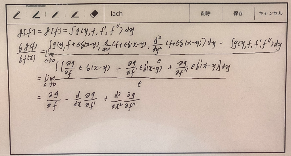
Table of Contents

## The Problem Statement

Consider a functional $J[f]$ defined as:

$J[f] = \int g\left(y, f, f^{\prime}, f^{\prime \prime}\right) \mathrm{d} y$

We are tasked with showing that:

$\frac{\delta J[f]}{\delta f(x)}=\frac{\partial g}{\partial f}-\frac{\mathrm{d}}{\mathrm{d} x} \frac{\partial g}{\partial f^{\prime}}+\frac{\mathrm{d}^2}{\mathrm{~d} x^2} \frac{\partial g}{\partial f^{\prime \prime}}$

Here, $f^{\prime \prime}$ is the second derivative of $f$ with respect to $y$ .

## The Solution Journey

### Step 1: Variational Notation

Let’s start by considering a small variation $\epsilon \delta(x-y)$ in the function $f(x)$ . The change $\delta J[f]$ in the functional $J[f]$ can then be expressed as:

$\delta J[f] = \lim_{{\epsilon \rightarrow 0}} \int \left[ g(y, f + \epsilon \delta(x-y), f^\prime, f^{\prime \prime}) - g(y, f, f^\prime, f^{\prime \prime}) \right] \mathrm{d} y$

### Step 2: Expanding the Functional

To simplify this further, we can expand $g$ using a Taylor series around $\epsilon = 0$ :

$g(y, f + \epsilon \delta(x-y), f^\prime, f^{\prime \prime}) \approx g(y, f, f^\prime, f^{\prime \prime}) + \epsilon \frac{\partial g}{\partial f} \delta(x-y) + \epsilon \frac{\partial g}{\partial f^\prime} \delta^\prime(x-y) + \epsilon \frac{\partial g}{\partial f^{\prime \prime}} \delta^{\prime \prime}(x-y)$

### Step 3: The Final Derivation

After substituting this expansion back into the expression for $\delta J[f]$ and taking the limit $\epsilon \rightarrow 0$ , we arrive at:

$\frac{\delta J[f]}{\delta f(x)} = \frac{\partial g}{\partial f} - \frac{\mathrm{d}}{\mathrm{d} x} \frac{\partial g}{\partial f^{\prime}} + \frac{\mathrm{d}^2}{\mathrm{d} x^2} \frac{\partial g}{\partial f^{\prime \prime}}$

## The Quantum Epilogue

What we’ve accomplished here is akin to deciphering a piece of the quantum code that describes the universe. The equation we’ve derived is more than a mere mathematical curiosity—it’s a lens that allows us to glimpse into the fascinating interplay of functionals and derivatives in the realm of QFT. It tells us how a small change in $f(x)$ can propagate through the entire functional landscape.

The same methodology applied here extends to many other problems in quantum field theory, solidifying our understanding of the universe, one functional derivative at a time.